Report
Executive Summary
Overview
The impact of government tax programs on neighborhood change is an evaluation process undertaken to assess the effect of NMTC and LIHTC government programs implemented in distressed communities to help elevate communities from poverty. When imagining the future on a large scale, the first to come to mind are futuristic buildings, flying cars, and new forms of technology. On a smaller scale, the future comes from neighborhood change. Our goal, as a team, is to analyze neighborhood change between 2000 and 2010 using Census data. Once we look at the changes that have occurred, we can evaluate programs we believe are essential to revitalizing communities. Specifically, we will evaluate if governmental programs, such as NMTC and LIHTC, successfully facilitate economic development in distressing communities.
Data
The evaluation team analyzes 1990 to 2010 census data from the Longitudinal Tabulated Database (LTDB) to identify neighborhood change, predict changes in identified neighborhoods, and use statistical models to show the effect of interventions undertaken by NMTC and LIHTC programs.
Methods
The evaluation team organized the evaluation process into six parts. Each of the parts identified and analyzed a specific output. The team looks at the introduction of the project and data management in parts one and two of the evaluation steps. The evaluation team further analyzed neighborhood change and presented descriptive statistics on changes in the neighborhood Median Household Value (MHV) from 2000 to 2010. At the end of the analysis of the LTDB data set used, the team predicted changes in MHV and used models to determine the effectiveness of NMTC and LIHTC programs.
Results
The analysis results show 23% growth across all the tracts regardless of whether they participated in the LIHTC program. However, the tracts that participated in the LIHTC program have 0.01% growth which has no statistically significant. Compared to the NMTC, findings show that tracts that participated in the NMTC got more growth and were statistically significant even though the R2 and the standard error for tracts that participated in the NMTC and LIHTC are the same..
Literature Review
You can access the literature out team reviewed here: Literature Review
Part I: Neighborhood Change
In order to determine the neighborhood change, the team calculates the Change in Median Household Value (MHV) between 2000 to 2010 and measures gentrification between 2000 and 2010. The team also picked Pittsburgh city in Pennsylvania, and visualized gentrification data points across the city.
Metrics
Data Sources
The evaluation team uses the LTDB data set for 2000 and 2010 and the LTDB metadata to identify neighborhood change. The team conducted data cleaning and identified common variables across the data set. The first data set includes variables from the long form of the census, while the second data set contains variables from the short version of the census. Regarding RAW data, the team was mindful and cautious of variable names and formats because they could cause an error to the entire project. Once variables were set, the team conducted DATA WRANGLING to clean up the data, merge files, and filter variables needed for the analysis.
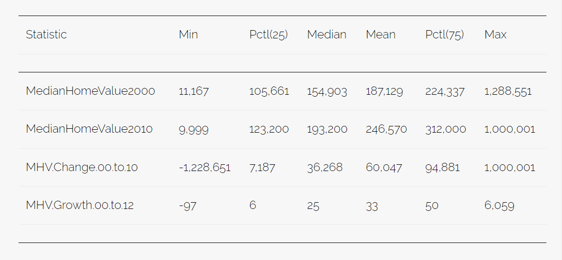
Median Home Value
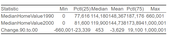
The Change in Median Home Value from 1990 to 2000 shows that the mean for 1990 and 2000 in monetary value is $3,629, which further shows a $3,629 standard deviation to the right of the mean on a bell curve. The findings also show that the middle point value between 1990 and 2000 is $453, as shown below.
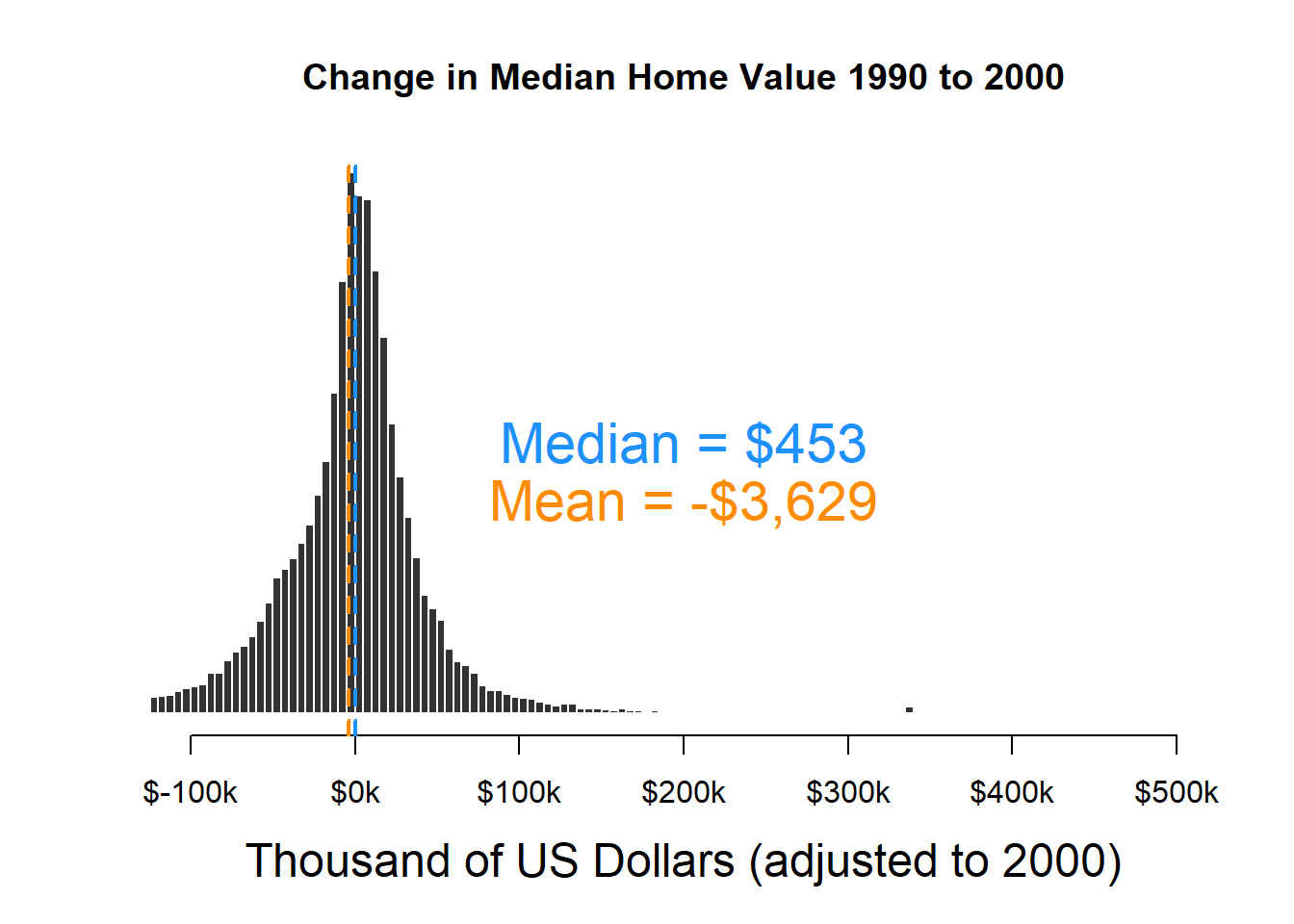
The figure below shows the level of growth change between 1990 and 2000. As indicated below, the result shows a 5% growth change between 1990 and 2000. Moreover, a zero median shows the midpoint between 1990 and 2000.

Gentrification
Gentrification as a social concept started in 1963 by a British Sociologist (Maciag, 2015). According to Herriges (2019), gentrification is a process through which cities change, and it helps to know who benefits from the changes that cities go through.
However, The variables the evaluation team selected to measure gentrification were home value in a lower-than-average home in a metro in 2000, above average diversity for a metro area, home value increase change in percentile rank within a metro area, faster than average home value rise, and increase in the proportion of whites. The team thought these variables would be an excellent way to identify areas where growth occurred with little to no displacement of minorities.
Descriptive Analysis of Neighborhood Change
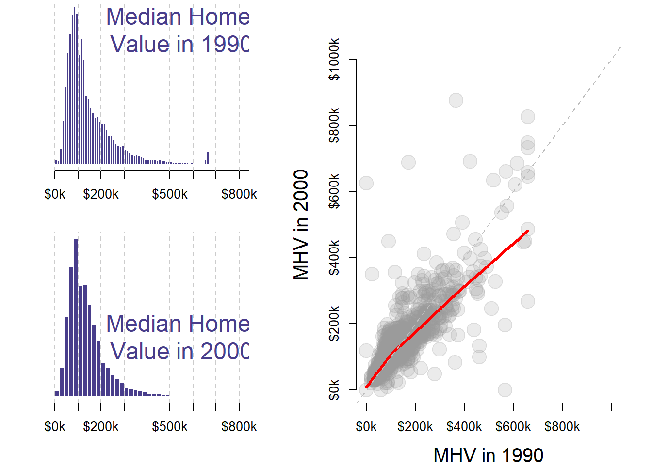
The initial conditions for MHV in 1990-2000
Average change in MHV 2000 to 2010
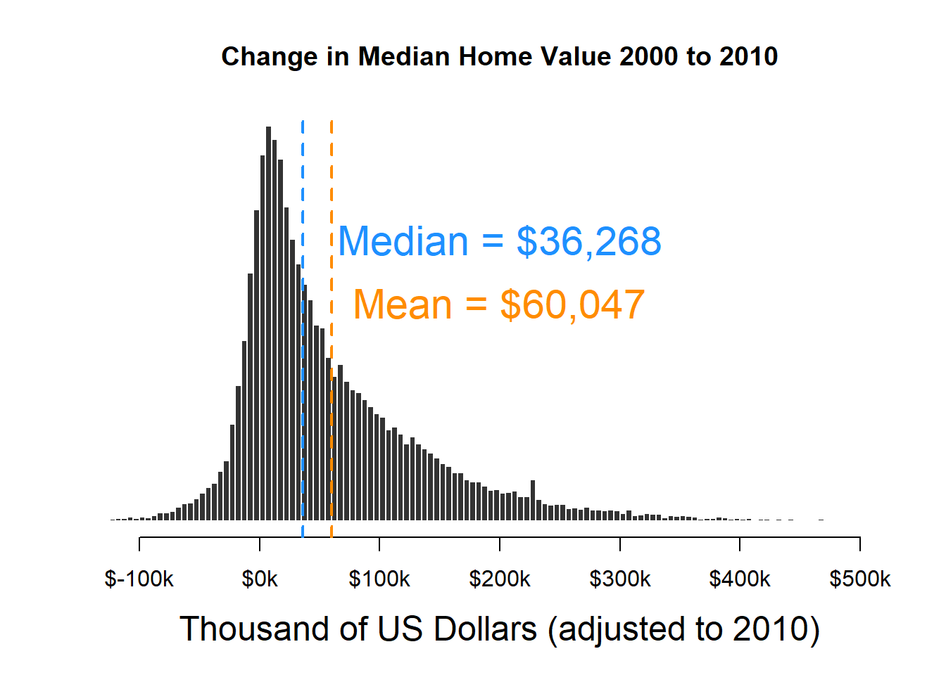
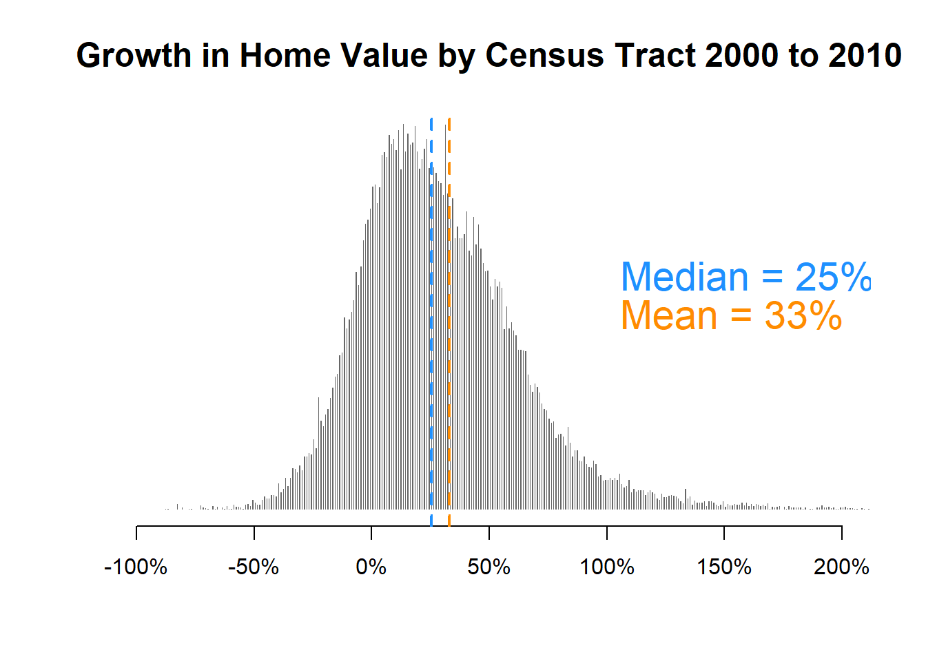
Comparing the median home value between 1990-2000 and 2000-2010. the analysis shows that 2000-2010 has a high median home value compared to 1990-2000. The Median Home Value from 2000-2010 is $35815 more than in 1990-2000. The Change in Median Home value from 2000-2010 is 28%, more than in 1990-2000, indicating a massive MHV growth rate for the years reviewed.
Predicting Change Based on 2000 Neighborhood Characteristics
In order to predict the median home value change Based on 2000, the team selected the following variables: The percentage of the black Population (p.black), the Percentage of the Population with a high school degree (p.hs), and the Percentage of the Population that is unemployed (p.unemp). However, the primary purpose for selecting the above variables is to assess how the variable affects the median home value change. Before running a model for the three variables selected, the team checked for variable skew and multicollinearity among the selected variables and the Media Home Value change for the 2000 and 2010 datasets. Since it is typical for social science data not to be normally distributed, the team conducted a formal testing of the variables selected to assess if there is any skew in the variables, as shown below.
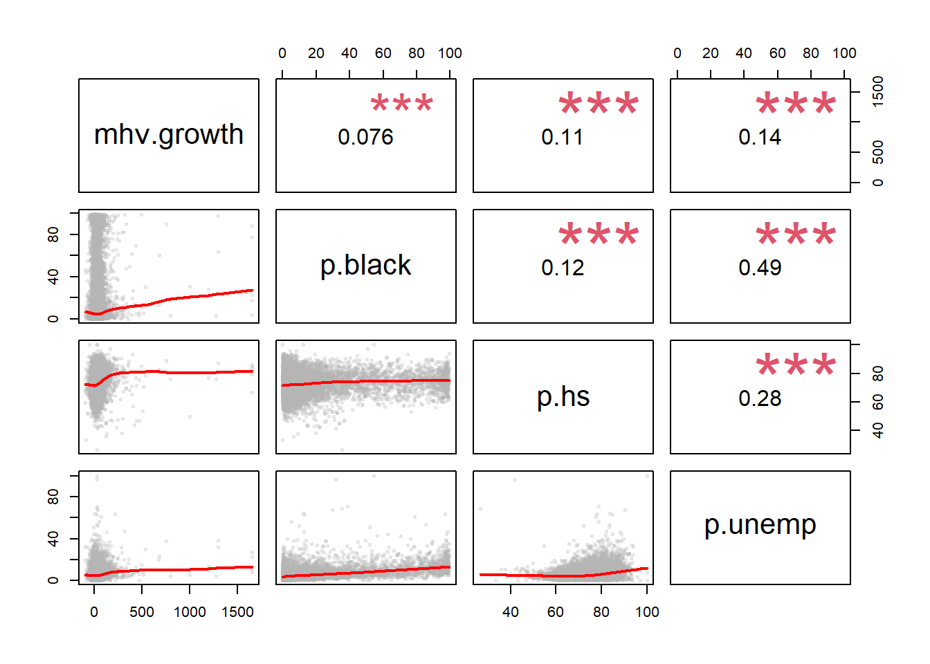
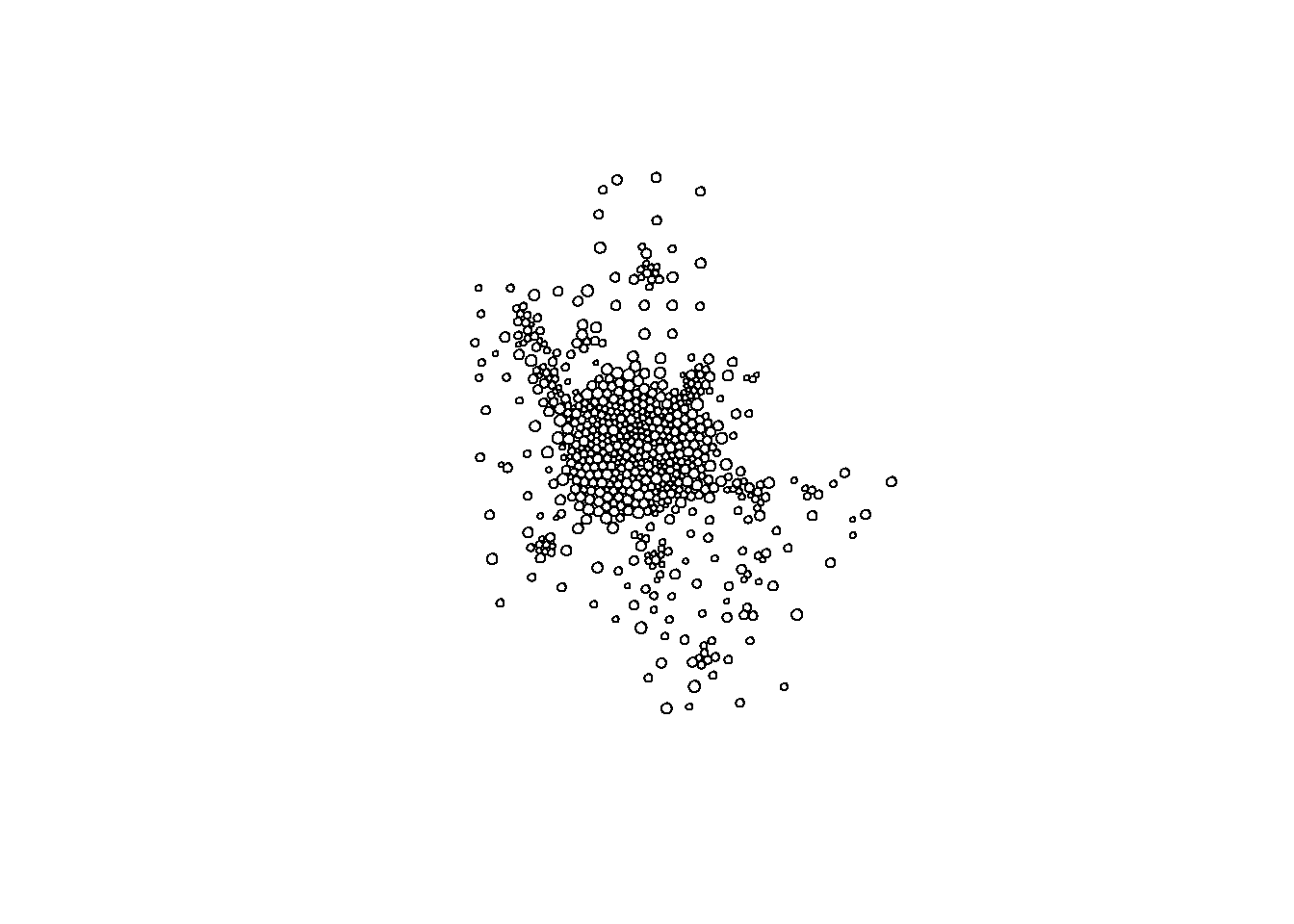
The relationship between selected variables in the scatter plot shows a cluster in the lower left-hand corner of the scatter plots, which shows evidence of skew data concerning MHV growth.
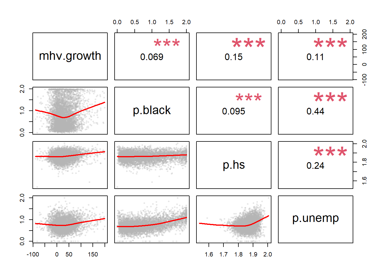
In addressing the skew in the variables in correlation to MHV growth, a log transformation was applied, which increased the level of correlation among the variable.
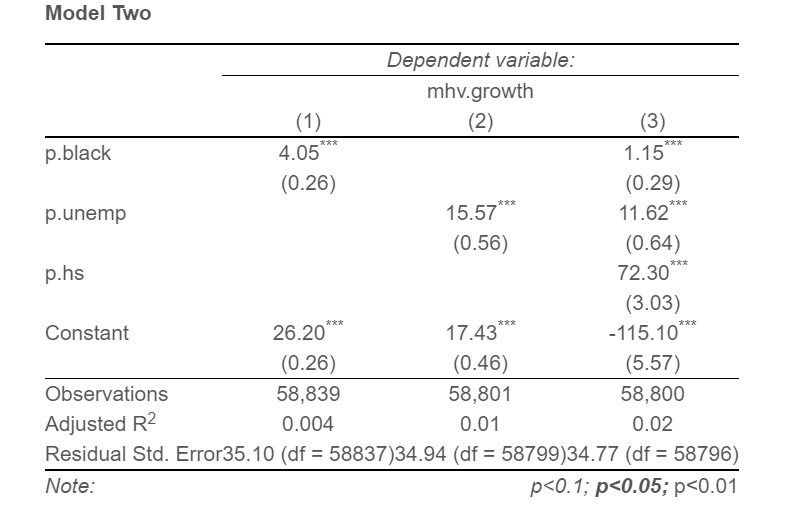
Even though all the variables are statistically significant, the following conclusions can be observed.
-
Coefficients for the black, unemployed population decrease
-
Standard errors increase for all the variables
-
Decrease in R-square across the model
-
Increase in Residual Std. Error in the model
The increase in the standard error in the model shows the distance of the data point to the regression line, affecting the model’s accuracy. The analysis suggests that the variables selected contain unwanted information, and including them together results in canceling each other out leads to a less effective model. In order to account for the context that may be responsible for the skew, the metro-level fixed effect is added to the model.
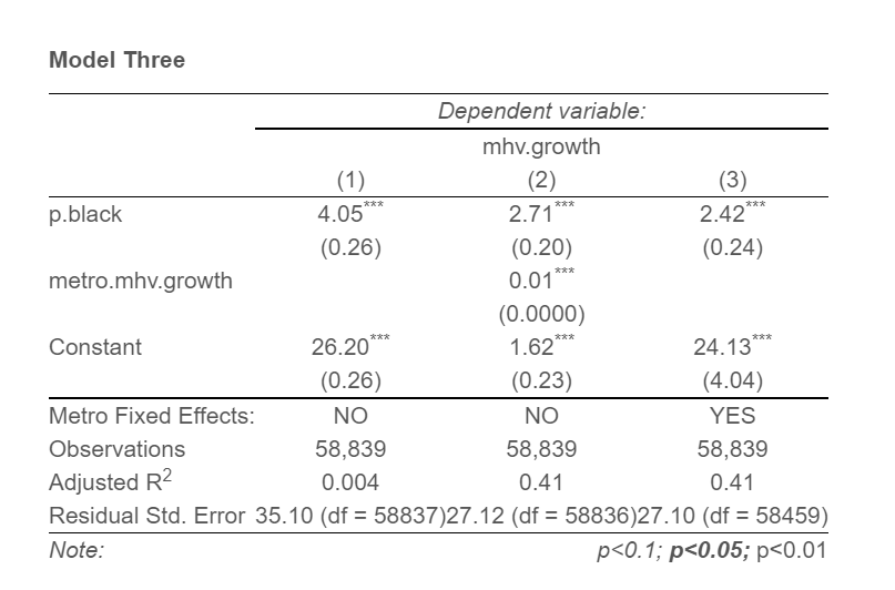
However, the relationship between the three variables (black population, unemployment population, and high school degree population) and Home Value Growth Change is positive and statistically significant. We can conclude that these three variables have an effect on MHV Growth. Moreover, the black population is considered the most critical variable among the three variables used to predict MHV change. After running models two and three, the black population remains statistically significant, and the standard error reduces.
Neighborhood Demographics
Spatial Characteristics (population density, adjacent tracts)
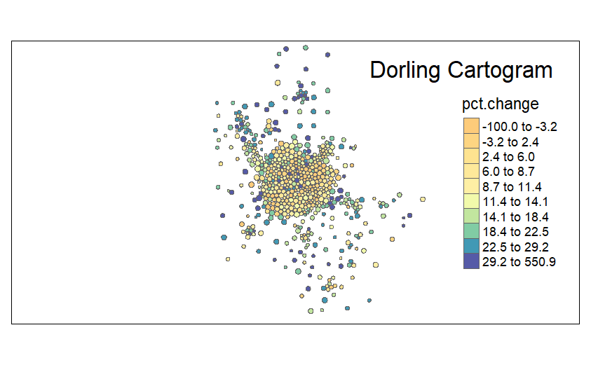
The dorling cartogram shows the census data and groups from clustering
The cartogram below shows the distribution of gentrification across the city. The map shows that change in the median home value happens more in the north and north-east of the city.
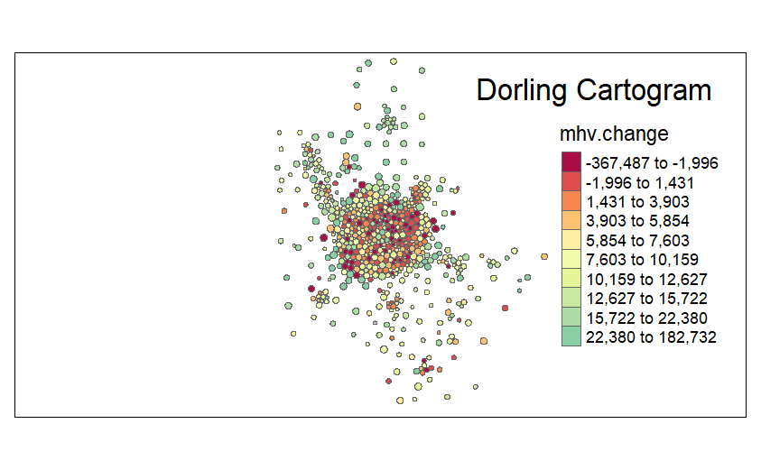
The cartogram below shows that the change in median home value as a result of the distribution of gentrification happens more in the north.
Part II: Evaluation of Tax Credits
Overview of Programs
New Market Tax Credits
The NMTC program helps economically distressed communities to influence private investment capital. The NMTC program provides investors with federal tax credits after meeting statutory qualifications. NMTC investment programs are expected to be implemented in a low-income neighborhoods.
Low Income Housing Tax Credits
Over the years, the government of the United States has used the Low Income Housing Tax Credit (LIHTC) to create affordable housing. The HUD made LIHTC available to the public in 1997, and the data sets have information on 47,511 projects and 3,13 million housing units between 1987 and 2017.
Data Manifest
The sample data set of 2000 has 72693 rows, the same as the complete data set, which shows a difference between the sample data set and the complete data set. In the case of the 2010 data set, the sample data set have 73056 while the complete data set has 72693, which means there are more threats in the 2010 full data set as compared to the sample data set for 2010. Also, the rodeo data set for 2000 has 72693 rows, showing that all the data sets in the complete data set are included in the sample data set. Moreover, the row of the rodeo data set for 2010 is 74022, which shows that the rows in the full data set are different from the sample data set because the margins in the 2010 data set the number of rows increases in the rodeo data set. However, from the 2000 data set, it is observed that all the counts are the same, meaning there are no changes in the data set. The completed data set differs from the rodeo data sets for 2000 and 2010, resulting from the many steps taken during the analysis. During the analysis, we filtered out row tracts for rural and maintained urban tracts and all the row tracts for Median Home Value for 2000 that are less than 10000. The series of adjustments reduces the number of rows for completed rodeo data set compared to the rodeo data set for 2000 and 2010.
Descriptive Statistics
Characteristics of neighborhoods that received them
The NMTC and LIHTC are great projects, but both projects have different eligibility criteria. The NMTC project enables economically distressed neighborhoods to access private investment capital using federal tax credits. On the other hand, the LIHTC project is not tied to census tracts but developers to make an available number of unities to qualified households.
The recipients of NMTC are poor and economically distressed communities. In the case of LIHTC, for you to benefit from the project, you have to build affordable housing units in poor communities.
Characteristics of those that did not
In the case of the NMTC project, only poor communities are targeted by the project, meaning communities that are not classified as poor would not benefit from the project.
On the other hand, LIHTC projects do not target a particular community or people. Instead, the project builds affordable housing units which are open to everyone.
Predictive Analysis
Aggregate average credits recieved between 2000 and 2010
The average number of tracts that received the LIHTC from 2010 to 2010 is 47302.67, and the ones that received the NMTC is 35792.88. The aggregate average tract that received credit from NMTC and LIHTC is 83095.55.
Update models by adding tax credit amounts
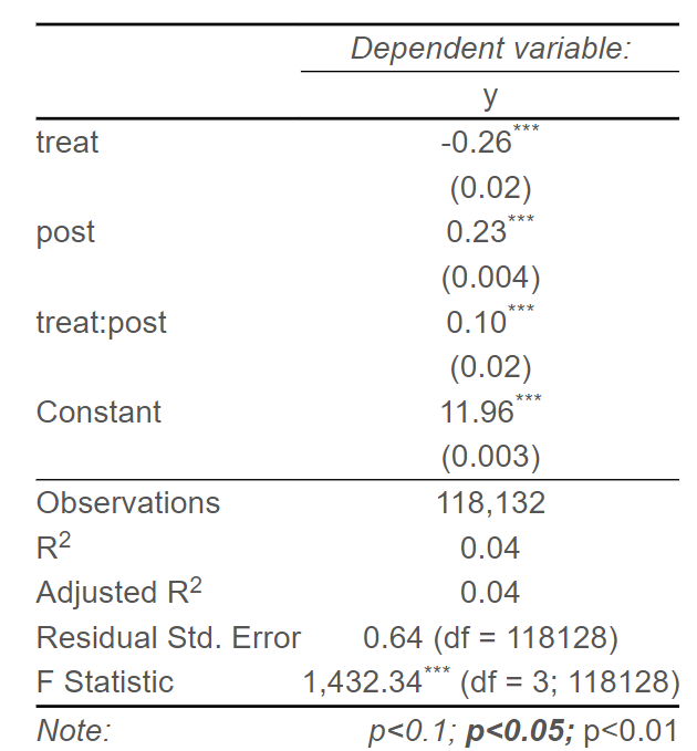
The model below shows the effect of NMTC on the identified neighborhood.
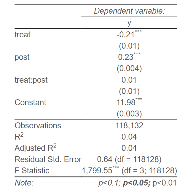
The model below shows the effect of LIHTC on the identified neighborhood.
Part III: Results and Conclusion
This evaluation aims to analyze neighborhood change between 2000 and 2010 using census data from the Longitudinal Tabulated Database (LTDB) to identify neighborhood change, predict changes in identified neighborhoods, and use statistical models to show the effect of interventions undertaken by NMTC and LIHTC programs.
The evaluation team organized the evaluation process into six parts. Each of the parts identified and analyzed a specific output. Further used the Difference-in-Difference Model to show the effects of the project’s interventions.
The findings indicate a 23% growth across all the tracts regardless of whether they participated in the NMTC program. However, the tracts participating in the NMTC program have 10% growth. In the case of the LIHTC program, the findings indicate a 23% growth across all the tracts regardless of whether they participated in the LIHTC program. However, the tracts that participated in the LIHTC program have 0.01% growth which is not statistically significant. Compared to the NMTC, it is observed that tracts that participated in the NMTC got more growth and were statistically significant.