Results and Conclusions

Introduction

The Centers for Disease Control and Prevention (CDC) Social Vulnerability Index (SVI) is an indicator to help identifying communities that may need extra support during emergencies. It is calculated from factors that represent the community poverty, unemployment, lack of education, age, disability, minority status, language barriers, crowded housing, and lack of transportation. The SVI ranges from 0 (least vulnerable) to 1 (most vulnerable).

Data

The Social Vulnerability Index (SVI) data used in this project originated from the CDC/ATSDR and was pulled at the census tract level for 2010 and at the Census Block Group (CBG) level for 2020. Since our analysis focused on tract-level comparisons over time, the 2020 SVI data were cross-walked to 2010 tract boundaries using the NHGIS geographic crosswalk, ensuring consistency in spatial units across both datasets.

Nationally, the raw 2010 SVI dataset included 73057 tracts. The 2020 dataset contained also 73057 tracts after cross-walking. Within the Mountain Division, there were 5250 tracts in 2010, and 5250 tracts in 2020.

We ranked the Mountain Division tracts by total number of flags. With this criteria, we found the most vulnerable tract in Laramie County, WY; and the least vulnerable, in Summit County, UT. While tract-level data may help identify pockets of need, counties serve as practical operational units for coordination and strategic planning.

The overall social vulnerability at the county level can be assessed from the complementary points of view of per-capita vulnerability and overall burden. First, we calculated the number of vulnerability flags per capita for each county. This method helps to identify counties with a population that face a high share of vulnerability, with a high per-capita social risk broadly distributed among residents. Second, we calculated the total number of vulnerability flags across all tracts in each county, which reflects the overall burden of vulnerability for the county. This approach emphasizes cumulative risk for counties with a large absolute number of vulnerable areas, regardless of how the vulnerability is concentrated across the population.

The counties with the highest widespread social vulnerability (measured as flags per capita) in 2010 were:

1. Clark County, ID . Pop: 857; Per Capita: 0.0082; Percentile (Per Capita): 100%; Total Flags: 7; Percentile (Total): 40%\
2. Esmeralda County, NV. Pop: 892; Per Capita: 0.0056; Percentile (Per Capita): 100%; Total Flags: 5; Percentile (Total): 40%\
3. Petroleum County, MT. Pop: 598, Per Capita: 0.0050, Percentile (Per Capita): 100%, Total Flags: 3, Percentile (Total): 20%)\

Each of these counties contain only a single census tract. In this case tract-level data and county-level reporting are functionally equivalent. All these three counties are extremely rural, sparsely populated and score poorly across multiple SVI dimensions. All all vulnerability flags assigned to that single tract are aggregated directly to the county level, and represent a relatively small number of residents; as a result, these counties appear highly vulnerable in terms of both total burden and per capita measures.

The counties with the highest overall vulnerability burden (measured as total flag count) were:

1. Maricopa County, AZ. Pop: 3,746,974; Total Flags: 3933; Percentile (Total): 100%; Per Capita: 0.0010; Percentile (Per Capita): 60%\
2. Clark County, NV. Pop: 1,895,521; Total Flags: 2433; Percentile (Total): 100%; Per Capita: 0.0013; Percentile (Per Capita): 80%\
3. Pima County, AZ. Pop: 960,309; Total Flags: 1113; Percentile (Total): 100%; Per Capita: 0.0012; Percentile (Per Capita): 80%.

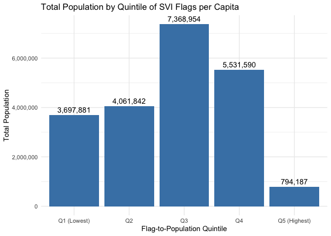
A representation of the aggregated distribution of population by Flag-to-Population Quintile reveals that counties in the highest quintile of per-capita vulnerability account for relatively few people, while middle-quintile counties represent the vast majority of the population in the Mountain Division. In fact, the counties in the top quintile of flags per capita include fewer than one million residents, compared to over seven million in the third quintile alone. This indicates that high flag-to-population ratios often occur in low-population counties where small denominators inflate per-capita metrics. Thus, while per-capita measures are useful for identifying disproportionately burdened areas, they should be complemented with absolute burden and population-size perspectives.

Mountain Division Population by SVI Quintile

In addition to the Social Vulnerability Index (SVI), the project incorporated several economic indicators to assess structural disadvantage and financial precarity at the census tract level. The House Price Index (HPI) tracks changes in residential property values over time and serves as a measure of housing market trends and cost burdens. HPI data were sourced from the Federal Housing Finance Agency (FHFA), which publishes regional indices reflecting inflation-adjusted home price changes (Federal Housing Finance Agency 2023). The analysis also used tract-level data on Median Household Income (MHI) and Median Home Value (MHV), obtained from the American Community Survey (ACS) 5-Year Estimates, published by the U.S. Census Bureau. These indicators helped contextualize economic vulnerability by identifying areas with low income levels or disproportionately high housing costs, both of which are key determinants of long-term economic insecurity (U.S. Census Bureau 2023).

The New Markets Tax Credit (NMTC) program was established to attract private investment to low-income communities by offering tax credits to investors who make equity investments in qualified Community Development Entities (CDEs). Census tracts qualify for NMTC allocation if they meet criteria indicating economic distress—most commonly a poverty rate of at least 20% or median family income at or below 80% of the area median income (AMI). Additional eligibility provisions include tracts with high unemployment, low home ownership rates, or located in designated high migration rural counties. These criteria are defined by the U.S. Department of the Treasury through the Community Development Financial Institutions Fund (CDFI Fund) and are designed to ensure that investment is directed toward areas with clear economic need (U.S. Department of the Treasury, Community Development Financial Institutions Fund 2023).

We have added to the NMTC-qualifying criteria the variables 20-year County population loss (from the 1990-2010 census), and the ratio Median Family Income (MFI) / Area Income 2011-2015 (between 80%-85% MFI). A tract with a % MFI / Area Income between 80% and 85% and evidence of demographic loss likely reflects a community in early-stage decline. While it may not yet meet federal thresholds, continued population loss is likely to depress income further, eventually qualifying it as distressed under programs like NMTC and LIHTC (Group 2018). Including population loss as an eligibility criterion for the New Markets Tax Credit (NMTC) program would enhance its ability to target communities facing long-term structural decline. While current criteria focus on poverty rates and income thresholds, these measures may overlook areas where population decline signals compounding challenges—such as business disinvestment, school closures, and service gaps that are not captured in static poverty data (Economic Innovation Group 2017; U.S. Department of the Treasury 2022). Many rural and post-industrial regions with shrinking populations lack the capacity to recover without external support. Expanding NMTC criteria to reflect population loss would align the program with broader federal goals to revitalize “left-behind” places (Muro and Maxim 2021b, 2021a).

The Low-Income Housing Tax Credit (LIHTC) program, administered by the Internal Revenue Service and the U.S. Department of Housing and Urban Development (HUD) seeks to promote the construction and rehabilitation of affordable rental housing. Eligibility for LIHTC incentives often focuses on Qualified Census Tracts (QCTs) and Difficult Development Areas (DDAs). QCTs are defined as census tracts where either 50% or more of households have incomes below 60% of AMI, or the poverty rate exceeds 25%. DDAs are areas where housing construction costs are high relative to income levels. These geographic designations play a key role in determining where enhanced credit allocations can be used, helping to channel affordable housing resources into the areas of greatest need (U.S. Department of Housing and Urban Development 2023a, 2023b).

In the Mountain Division, of a total of 1938 NMTC-eligible tracts 141 received NMTC project awards; and of a total of 202 LIHTC-eligible tracts 25 received LIHTC allocations.

A Core-Based Statistical Area (CBSA) is a geographic unit defined by the U.S. Office of Management and Budget (OMB) based on urban population centers and commuting patterns. CBSAs include both Metropolitan Statistical Areas (urban cores of 50,000+ people) and Micropolitan Statistical Areas (urban cores of 10,000–49,999 people) (OMB, 2023). In programs like the New Markets Tax Credit (NMTC) and the Low-Income Housing Tax Credit (LIHTC), CBSAs are used to define Area Median Income (AMI), which serves as a benchmark for determining eligibility and affordability thresholds (U.S. Department of Housing and Urban Development 2023a). By using CBSA-level AMI instead of national figures, these programs help control for metro-level effects—ensuring that income and poverty comparisons reflect local economic conditions rather than national averages. For example, a household making $60,000 may be considered low-income in a high-cost metro like Denver, but middle-income in rural Montana. CBSA-based benchmarks allow programs like NMTC and LIHTC to better identify economically distressed areas in both urban and rural contexts (Group 2018; Economic Innovation Group 2017)

Analysis

To examine the relationship between vulnerability and federal investment, we created bivariate choropleth maps that visualized both the overall vulnerability burden and the dollar amounts awarded through NMTC and LIHTC programs. These maps allowed us to highlight areas where high need aligned with high investment, as well as places where funding may be lacking despite significant vulnerability. The spatial tools were essential for identifying geographic disparities and suggesting potential gaps in resource allocation.

To better understand relationships among variables, we conducted correlation analyses. These tests helped quantify the associations between different measures of vulnerability, such as the relationship between population size, total flag count, and median income. We applied k-means clustering to categorize counties based on their total vulnerability burden (flag count) and the dollar amount of NMTC and LIHTC awards received. This method allowed us to detect patterns across the region by grouping counties with similar combinations of need and investment, and draw attention to mismatches between social need and resource allocation.

Finally, to examine how investment or eligibility status may be associated with changes over time, we implemented a difference-in-differences (diff-in-diff) regression analysis. This quasi-experimental method compared changes in outcomes—such as economic or housing indicators—between counties that qualified for federal investment (e.g., LIHTC or NMTC) and those that did not, before and after a given policy window. By controlling for baseline differences and time trends, this approach provided a more rigorous estimate of program impacts than simple before-and-after comparisons.

Results

NMTC Diff-In-Diff Models

Socioeconomic SVI

We fitted a linear model (estimated using OLS) to predict SVI_FLAG_COUNT_SES with treat, post and cbsa (formula: SVI_FLAG_COUNT_SES ~ treat + post + treat * post + cbsa) where treat represents NMTC program participation, post is the year of 2020 after starting period of 2010, and cbsa controls for metro-level effects.

The model explains a statistically significant and moderate proportion of variance (R2 = 0.18, F(75, 3360) = 10.16, p < .001, adj. R2 = 0.17)

The effect of treat × post is statistically non-significant and positive (beta = 0.02, 95% CI \(-0.35, 0.39\), t(3360) = 0.11, p = 0.914; Std. beta = 1.68e-03, 95% CI \(-0.03, 0.03\))

Since the effect of treat x post is not statistically significant, we cannot conclude that the NMTC program had a measurable impact on socioeconomic status-related social vulnerability and economic outcomes.

Household Characteristics SVI

We fitted a linear model (estimated using OLS) to predict SVI_FLAG_COUNT_HHCHAR with treat, post and cbsa (formula: SVI_FLAG_COUNT_HHCHAR ~ treat + post + treat * post + cbsa) where treat represents NMTC program participation, post is the year of 2020 after starting period of 2010, and cbsa controls for metro-level effects.

The model explains a statistically significant and moderate proportion of variance (R2 = 0.19, F(75, 3360) = 10.28, p < .001, adj. R2 = 0.17)

The effect of treat × post is statistically non-significant and positive (beta = 4.92e-03, 95% CI \(-0.25, 0.26\), t(3360) = 0.04, p = 0.970; Std. beta = 5.86e-04, 95% CI \(-0.03, 0.03\))

Since the effect of treat x post is not statistically significant, we cannot conclude that the NMTC program had a measurable impact on household characteristics-related social vulnerability and economic outcomes.

Racial and Ethnic Minority SVI

We fitted a linear model (estimated using OLS) to predict SVI_FLAG_COUNT_REM with treat, post and cbsa (formula: SVI_FLAG_COUNT_REM ~ treat + post + treat * post + cbsa) where treat represents NMTC program participation, post is the year of 2020 after starting period of 2010, and cbsa controls for metro-level effects.

The model explains a statistically significant and substantial proportion of variance (R2 = 0.34, F(75, 3360) = 23.24, p < .001, adj. R2 = 0.33)

The effect of treat × post is statistically non-significant and negative (beta = -4.57e-03, 95% CI \(-0.11, 0.10\), t(3360) = -0.09, p = 0.932; Std. beta = -1.19e-03, 95% CI \(-0.03, 0.03\))

Since the effect of treat x post is not statistically significant, we cannot conclude that the NMTC program had a measurable impact on racial and ethnic minority status-related social vulnerability and economic outcomes.

Housing and Transportation SVI

We fitted a linear model (estimated using OLS) to predict SVI_FLAG_COUNT_HOUSETRANSPT with treat, post and cbsa (formula: SVI_FLAG_COUNT_HOUSETRANSPT ~ treat + post + treat * post + cbsa) where treat represents NMTC program participation, post is the year of 2020 after starting period of 2010, and cbsa controls for metro-level effects.

The model explains a statistically significant and weak proportion of variance (R2 = 0.11, F(75, 3360) = 5.71, p < .001, adj. R2 = 0.09)

The effect of treat × post is statistically non-significant and positive (beta = 0.09, 95% CI \(-0.19, 0.36\), t(3360) = 0.62, p = 0.537; Std. beta = 0.01, 95% CI \(-0.02, 0.04\))

Since the effect of treat x post is not statistically significant, we cannot conclude that the NMTC program had a measurable impact on housing and transportation access-related social vulnerability and economic outcomes.

Overall SVI

We fitted a linear model (estimated using OLS) to predict SVI_FLAG_COUNT_OVERALL with treat, post and cbsa (formula: SVI_FLAG_COUNT_OVERALL ~ treat + post + treat * post + cbsa) where treat represents NMTC program participation, post is the year of 2020 after starting period of 2010, and cbsa controls for metro-level effects.

The model explains a statistically significant and moderate proportion of variance (R2 = 0.24, F(75, 3360) = 13.76, p < .001, adj. R2 = 0.22)

The effect of treat × post is statistically non-significant and positive (beta = 0.11, 95% CI \(-0.64, 0.85\), t(3360) = 0.28, p = 0.779; Std. beta = 4.23e-03, 95% CI \(-0.03, 0.03\))

Since the effect of treat x post is not statistically significant, we cannot conclude that the NMTC program had a measurable impact on socioeconomic, household characteristics, racial and ethnic minority status, and housing and transportation access-related social vulnerability and economic outcomes.

Median Income Economic Outcomes

We fitted a linear model (estimated using OLS) to predict MEDIAN_INCOME with treat, post and cbsa (formula: MEDIAN_INCOME ~ treat + post + treat * post + cbsa) where treat represents NMTC program participation, post is the year of 2020 after starting period of 2010, and cbsa controls for metro-level effects.

The model explains a statistically significant and moderate proportion of variance (R2 = 0.22, F(75, 3360) = 12.43, p < .001, adj. R2 = 0.20)

The effect of treat × post is statistically non-significant and positive (beta = 1.24e-15, 95% CI \(-0.07, 0.07\), t(3360) = 3.50e-14, p > .999; Std. beta = -3.14e-16, 95% CI \(-0.03, 0.03\))

Since the effect of treat x post is not statistically significant, we cannot conclude that the NMTC program had a measurable impact on Median Income-related social vulnerability and economic outcomes.

Median Home Value Economic Outcomes

We fitted a linear model (estimated using OLS) to predict MEDIAN_HOME_VALUE with treat, post and cbsa (formula: MEDIAN_HOME_VALUE ~ treat + post + treat * post + cbsa) where treat represents NMTC program participation, post is the year of 2020 after starting period of 2010, and cbsa controls for metro-level effects.

The model explains a statistically significant and moderate proportion of variance (R2 = 0.20, F(75, 3300) = 11.10, p < .001, adj. R2 = 0.18)

The effect of treat × post is statistically non-significant and positive (beta = 3.17e-16, 95% CI \(-0.12, 0.12\), t(3300) = 5.17e-15, p > .999; Std. beta = -4.98e-17, 95% CI \(-0.03, 0.03\))

Since the effect of treat x post is not statistically significant, we cannot conclude that the NMTC program had a measurable impact on Median Home Value-related social vulnerability and economic outcomes.

House Price Index Economic Outcomes

We fitted a linear model (estimated using OLS) to predict HOUSE_PRICE_INDEX with treat, post and cbsa (formula: HOUSE_PRICE_INDEX ~ treat + post + treat * post + cbsa) where treat represents NMTC program participation, post is the year of 2020 after starting period of 2010, and cbsa controls for metro-level effects.

The model explains a statistically significant and substantial proportion of variance (R2 = 0.61, F(71, 1902) = 41.96, p < .001, adj. R2 = 0.60)

The effect of treat × post is statistically non-significant and negative (beta = -5.21e-04, 95% CI \(-0.11, 0.11\), t(1902) = -9.32e-03, p = 0.993; Std. beta = -1.33e-04, 95% CI \(-0.03, 0.03\))

Since the effect of treat x post is not statistically significant, we cannot conclude that the NMTC program had a measurable impact on House Price Index-related social vulnerability and economic outcomes.

LIHTC Diff-In-Diff Models

Socioeconomic SVI

We fitted a linear model (estimated using OLS) to predict SVI_FLAG_COUNT_SES with treat, post and cbsa (formula: SVI_FLAG_COUNT_SES ~ treat + post + treat * post + cbsa) where treat represents LIHTC program participation, post is the year of 2020 after starting period of 2010, and cbsa controls for metro-level effects.

The model explains a statistically significant and moderate proportion of variance (R2 = 0.26, F(39, 332) = 2.91, p < .001, adj. R2 = 0.17)

The effect of treat × post is statistically non-significant and negative (beta = -0.26, 95% CI \(-0.87, 0.35\), t(332) = -0.83, p = 0.406; Std. beta = -0.04, 95% CI \(-0.13, 0.05\))

Since the effect of treat x post is not statistically significant, we cannot conclude that the LIHTC program had a measurable impact on socioeconomic status-related social vulnerability and economic outcomes.

Household Characteristics SVI

We fitted a linear model (estimated using OLS) to predict SVI_FLAG_COUNT_HHCHAR with treat, post and cbsa (formula: SVI_FLAG_COUNT_HHCHAR ~ treat + post + treat * post + cbsa) where treat represents LIHTC program participation, post is the year of 2020 after starting period of 2010, and cbsa controls for metro-level effects.

The model explains a statistically significant and substantial proportion of variance (R2 = 0.43, F(39, 332) = 6.52, p < .001, adj. R2 = 0.37)

The effect of treat × post is statistically non-significant and negative (beta = -0.06, 95% CI \(-0.64, 0.53\), t(332) = -0.19, p = 0.847; Std. beta = -7.97e-03, 95% CI \(-0.09, 0.07\))

Since the effect of treat x post is not statistically significant, we cannot conclude that the LIHTC program had a measurable impact on household characteristics-related social vulnerability and economic outcomes.

Racial and Ethnic Minority SVI

We fitted a linear model (estimated using OLS) to predict SVI_FLAG_COUNT_REM with treat, post and cbsa (formula: SVI_FLAG_COUNT_REM ~ treat + post + treat * post + cbsa) where treat represents LIHTC program participation, post is the year of 2020 after starting period of 2010, and cbsa controls for metro-level effects.

The model explains a statistically significant and substantial proportion of variance (R2 = 0.59, F(39, 332) = 12.22, p < .001, adj. R2 = 0.54)

The effect of treat × post is statistically non-significant and negative (beta = -6.17e-03, 95% CI \(-0.20, 0.19\), t(332) = -0.06, p = 0.950; Std. beta = -2.23e-03, 95% CI \(-0.07, 0.07\))

Since the effect of treat x post is not statistically significant, we cannot conclude that the LIHTC program had a measurable impact on racial and ethnic minority status-related social vulnerability and economic outcomes.

Housing and Transportation SVI

We fitted a linear model (estimated using OLS) to predict SVI_FLAG_COUNT_HOUSETRANSPT with treat, post and cbsa (formula: SVI_FLAG_COUNT_HOUSETRANSPT ~ treat + post + treat * post + cbsa) where treat represents LIHTC program participation, post is the year of 2020 after starting period of 2010, and cbsa controls for metro-level effects.

The model explains a statistically significant and moderate proportion of variance (R2 = 0.20, F(39, 332) = 2.08, p < .001, adj. R2 = 0.10)

The effect of treat × post is statistically non-significant and positive (beta = 0.19, 95% CI \(-0.37, 0.75\), t(332) = 0.67, p = 0.503; Std. beta = 0.03, 95% CI \(-0.06, 0.13\))

Since the effect of treat x post is not statistically significant, we cannot conclude that the LIHTC program had a measurable impact on housing and transportation access-related social vulnerability and economic outcomes.

Overall SVI

We fitted a linear model (estimated using OLS) to predict SVI_FLAG_COUNT_OVERALL with treat, post and cbsa (formula: SVI_FLAG_COUNT_OVERALL ~ treat + post + treat * post + cbsa) where treat represents LIHTC program participation, post is the year of 2020 after starting period of 2010, and cbsa controls for metro-level effects.

The model explains a statistically significant and substantial proportion of variance (R2 = 0.42, F(39, 332) = 6.20, p < .001, adj. R2 = 0.35)

The effect of treat × post is statistically non-significant and negative (beta = -0.13, 95% CI \(-1.39, 1.12\), t(332) = -0.21, p = 0.837; Std. beta = -8.60e-03, 95% CI \(-0.09, 0.07\))

Since the effect of treat x post is not statistically significant, we cannot conclude that the LIHTC program had a measurable impact on socioeconomic, household characteristics, racial and ethnic minority status, and housing and transportation access-related social vulnerability and economic outcomes.

Median Income Economic Outcomes

We fitted a linear model (estimated using OLS) to predict MEDIAN_INCOME with treat, post and cbsa (formula: MEDIAN_INCOME ~ treat + post + treat * post + cbsa) where treat represents LIHTC program participation, post is the year of 2020 after starting period of 2010, and cbsa controls for metro-level effects.

The model explains a statistically significant and substantial proportion of variance (R2 = 0.38, F(39, 332) = 5.25, p < .001, adj. R2 = 0.31)

The effect of treat × post is statistically non-significant and negative (beta = -4.76e-16, 95% CI \(-0.23, 0.23\), t(332) = -4.09e-15, p > .999; Std. beta = -1.28e-16, 95% CI \(-0.09, 0.09\))

Since the effect of treat x post is not statistically significant, we cannot conclude that the LIHTC program had a measurable impact on Median Income-related social vulnerability and economic outcomes.

Median Home Value Economic Outcomes

We fitted a linear model (estimated using OLS) to predict MEDIAN_HOME_VALUE with treat, post and cbsa (formula: MEDIAN_HOME_VALUE ~ treat + post + treat * post + cbsa) where treat represents LIHTC program participation, post is the year of 2020 after starting period of 2010, and cbsa controls for metro-level effects.

The model explains a statistically significant and substantial proportion of variance (R2 = 0.43, F(39, 314) = 6.08, p < .001, adj. R2 = 0.36)

The effect of treat × post is statistically non-significant and negative (beta = -2.61e-16, 95% CI \(-0.30, 0.30\), t(314) = -1.71e-15, p > .999; Std. beta = -2.08e-17, 95% CI \(-0.08, 0.08\))

Since the effect of treat x post is not statistically significant, we cannot conclude that the LIHTC program had a measurable impact on Median Home Value-related social vulnerability and economic outcomes.

House Price Index Economic Outcomes

We fitted a linear model (estimated using OLS) to predict HOUSE_PRICE_INDEX with treat, post and cbsa (formula: HOUSE_PRICE_INDEX ~ treat + post + treat * post + cbsa) where treat represents LIHTC program participation, post is the year of 2020 after starting period of 2010, and cbsa controls for metro-level effects.

The model explains a statistically significant and substantial proportion of variance (R2 = 0.65, F(23, 102) = 8.41, p < .001, adj. R2 = 0.58)

The effect of treat × post is statistically non-significant and positive (beta = 0.03, 95% CI \(-0.37, 0.44\), t(102) = 0.17, p = 0.865; Std. beta = 9.99e-03, 95% CI \(-0.11, 0.13\))

Since the effect of treat x post is not statistically significant, we cannot conclude that the LIHTC program had a measurable impact on House Price Index-related social vulnerability and economic outcomes.

Discussion and Recommendations

This analysis examined the effects of the New Markets Tax Credit (NMTC) and Low-Income Housing Tax Credit (LIHTC) programs on measures of social vulnerability and economic outcomes using difference-in-differences (DiD) linear regression models. Each model included variables for treatment status, a post-intervention period (2020), and metropolitan area fixed effects (CBSA). The main parameter of interest was the interaction between treatment and the post-period (treat × post), which captures the estimated effect of program participation after 2010.

For the NMTC program, none of the interaction effects were statistically significant across any of the outcome areas. The models tested the program’s association with five CDC Social Vulnerability Index (SVI) themes (socioeconomic status, household characteristics, racial and ethnic minority status, housing and transportation access, and overall vulnerability) as well as three economic indicators (median income, median home value, and house price index). While several models demonstrated moderate to substantial explanatory power (e.g., R² = 0.34 for racial and ethnic SVI and R² = 0.61 for house price index), the absence of statistically significant treat × post effects indicates that NMTC program participation did not produce measurable improvements in the analyzed social or economic outcomes at the census tract level during the 2010–2020 period.

The findings for the LIHTC program followed a similar pattern. Across all five SVI domains and the three economic outcomes, no statistically significant interaction effects were found. Although the LIHTC models often explained a considerable proportion of variance (e.g. R² values of 0.59 for racial and ethnic SVI and 0.65 for the house price index) the program’s presence did not correspond to measurable post-2010 changes in the selected indicators. These results suggest that, within the scope of this analysis, LIHTC funding did not produce detectable tract-level effects on social vulnerability or economic development.

In this study, we assessed the impact of NMTC and LIHTC programs at the tract-level. Tracts give us detailed local information, but since some of the counties with the highest vulnerability scores only have one census tract and very small populations, they can heavily influence the results and may not reflect broader trends.

Further analysis at the county-level may provide complementary more robust, policy-relevant insights. Although it may mask important variations such as disparities between wealthier and poorer neighborhoods, aggregating data by county can reduce noise by smoothing out extreme values that often arise in small or sparsely populated tracts. This approach would better reflect that programs like NMTC and LIHTC are typically implemented across broader areas such as entire counties or metropolitan regions rather than isolated neighborhoods.

Currently, our models treat program participation as a simple yes-or-no variable—whether an area received NMTC or LIHTC funding or not. However, this approach overlooks a key detail: not all areas received the same amount of funding. Some may have received only small grants, while others benefited from much larger investments. Including the actual dollar amounts allocated to each area could provide more accurate and meaningful results, allowing us to see whether higher levels of funding are linked to better outcomes. This would also offer more useful guidance for policymakers by indicating how much funding is needed to create real impact, and it would allow for fairer comparisons between areas with vastly different funding levels. That said, using funding amounts comes with challenges. Areas that received more funding may already have had advantages—such as stronger local institutions or political support—which makes it difficult to separate the effect of the funding from other factors. To address this, more advanced methods would be needed to isolate the true impact of funding levels.

In conclusion, the analysis finds no evidence that either NMTC or LIHTC participation was associated with significant changes in the selected outcome variables over the study period. While model fits were generally strong and controlled for geographic variation, the binary treatment specification and tract-level scale may have limited the ability to detect more nuanced or longer-term effects. Future analyses may benefit from incorporating actual investment amounts, aggregating to the county level, or accounting for potential treatment lags in order to capture a fuller picture of these programs’ impacts.

References

R Version

Analyses were conducted using the R Statistical language (version 4.4.3; R Core Team, 2025) on macOS Sequoia 15.3.2

R Packages

• Arel-Bundock V (2022). “modelsummary: Data and Model Summaries in R.” Journal of Statistical Software, 103(1), 1-23. <doi:10.18637/jss.v103.i01> https://doi.org/10.18637/jss.v103.i01.
• Arel-Bundock V (2024). tinytable: Simple and Configurable Tables in ‘HTML’, ‘LaTeX’, ‘Markdown’, ‘Word’, ‘PNG’, ‘PDF’, and ‘Typst’ Formats. R package version 0.2.1, https://vincentarelbundock.github.io/tinytable/.
• Auguie B (2017). gridExtra: Miscellaneous Functions for “Grid” Graphics. R package version 2.3.
• Chan C, Leeper T, Becker J, Schoch D (2023). rio: A Swiss-army knife for data file I/O. https://cran.r-project.org/package=rio.
• Cheng J, Sievert C, Schloerke B, Chang W, Xie Y, Allen J (2023). htmltools: Tools for HTML. R package version 0.5.7, https://rstudio.github.io/htmltools/, https://github.com/rstudio/htmltools.
• Gagolewski M (2022). “stringi: Fast and portable character string processing in R.” Journal of Statistical Software, 103(2), 1-59. <doi:10.18637/jss.v103.i02> https://doi.org/10.18637/jss.v103.i02.
• Gohel D, Skintzos P (2024). ggiraph: Make ‘ggplot2’ Graphics Interactive. R package version 0.8.9, https://davidgohel.github.io/ggiraph/.
• Grolemund G, Wickham H (2011). “Dates and Times Made Easy with lubridate.” Journal of Statistical Software, 40(3), 1-25. https://www.jstatsoft.org/v40/i03/.
• Karambelkar B (2017). widgetframe: ‘Htmlwidgets’ in Responsive ‘iframes’. R package version 0.3.1, https://bhaskarvk.github.io/widgetframe/, https://github.com/bhaskarvk/widgetframe.
• Kassambara A (2023). ggpubr: ‘ggplot2’ Based Publication Ready Plots. R package version 0.6.0, https://rpkgs.datanovia.com/ggpubr/.
• Kassambara A, Mundt F (2020). factoextra: Extract and Visualize the Results of Multivariate Data Analyses. R package version 1.0.7, http://www.sthda.com/english/rpkgs/factoextra.
• Komsta L, Novomestky F (2022). moments: Moments, Cumulants, Skewness, Kurtosis and Related Tests. R package version 0.14.1, http://www.komsta.net/, https://www.r-project.org.
• Maechler M, Rousseeuw P, Struyf A, Hubert M, Hornik K (2023). cluster: Cluster Analysis Basics and Extensions. R package version 2.1.6 - For new features, see the ‘NEWS’ and the ‘Changelog’ file in the package source), https://CRAN.R-project.org/package=cluster.
• Makowski D, Lüdecke D, Patil I, Thériault R, Ben-Shachar M, Wiernik B (2023). “Automated Results Reporting as a Practical Tool to Improve Reproducibility and Methodological Best Practices Adoption.” CRAN. https://easystats.github.io/report/.
• Mangiafico SS (2024). rcompanion: Functions to Support Extension Education Program Evaluation. Rutgers Cooperative Extension, New Brunswick, New Jersey. version 2.4.35, https://CRAN.R-project.org/package=rcompanion/.
• Müller K (2020). here: A Simpler Way to Find Your Files. R package version 1.0.1, https://github.com/r-lib/here, https://here.r-lib.org/.
• Müller K, Wickham H (2023). tibble: Simple Data Frames. R package version 3.2.1, https://github.com/tidyverse/tibble, https://tibble.tidyverse.org/.
• Ooms J (2024). magick: Advanced Graphics and Image-Processing in R. R package version 2.8.3, https://docs.ropensci.org/magick/https://ropensci.r-universe.dev/magick.
• Pedersen T (2024). patchwork: The Composer of Plots. R package version 1.2.0, https://github.com/thomasp85/patchwork, https://patchwork.data-imaginist.com.
• Prener C, Grossenbacher T, Zehr A (2022). biscale: Tools and Palettes for Bivariate Thematic Mapping. R package version 1.0.0, https://chris-prener.github.io/biscale/.
• Qiu Y, details. aotifSfAf (2020). showtextdb: Font Files for the ‘showtext’ Package. R package version 3.0.
• Qiu Y, details. aotifSfAf (2024). sysfonts: Loading Fonts into R. R package version 0.8.9, https://github.com/yixuan/sysfonts.
• Qiu Y, details. aotisSfAf (2024). showtext: Using Fonts More Easily in R Graphs. R package version 0.9-7, https://github.com/yixuan/showtext.
• R Core Team (2023). R: A Language and Environment for Statistical Computing. R Foundation for Statistical Computing, Vienna, Austria. https://www.R-project.org/.
• Slowikowski K (2024). ggrepel: Automatically Position Non-Overlapping Text Labels with ‘ggplot2’. R package version 0.9.5, https://github.com/slowkow/ggrepel, https://ggrepel.slowkow.com/.
• Ushey K, Wickham H (2024). renv: Project Environments. R package version 1.0.5, https://CRAN.R-project.org/package=renv.
• Vaidyanathan R, Xie Y, Allaire J, Cheng J, Sievert C, Russell K (2023). htmlwidgets: HTML Widgets for R. R package version 1.6.4, https://github.com/ramnathv/htmlwidgets.
• Vidonne C, Dicko A (2023). unhcrthemes: UNHCR ‘ggplot2’ Theme and Colour Palettes. R package version 0.6.2, https://unhcr-dataviz.github.io/unhcrthemes/, https://github.com/unhcr-dataviz/unhcrthemes.
• Walker K (2024). tigris: Load Census TIGER/Line Shapefiles. R package version 2.1, https://github.com/walkerke/tigris.
• Walker K, Herman M (2024). tidycensus: Load US Census Boundary and Attribute Data as ‘tidyverse’ and ‘sf’-Ready Data Frames. R package version 1.6.2, https://walker-data.com/tidycensus/.
• Wickham H (2016). ggplot2: Elegant Graphics for Data Analysis. Springer-Verlag New York. ISBN 978-3-319-24277-4, https://ggplot2.tidyverse.org.
• Wickham H (2023). forcats: Tools for Working with Categorical Variables (Factors). R package version 1.0.0, https://github.com/tidyverse/forcats, https://forcats.tidyverse.org/.
• Wickham H (2023). stringr: Simple, Consistent Wrappers for Common String Operations. R package version 1.5.1, https://github.com/tidyverse/stringr, https://stringr.tidyverse.org.
• Wickham H, Averick M, Bryan J, Chang W, McGowan LD, François R, Grolemund G, Hayes A, Henry L, Hester J, Kuhn M, Pedersen TL, Miller E, Bache SM, Müller K, Ooms J, Robinson D, Seidel DP, Spinu V, Takahashi K, Vaughan D, Wilke C, Woo K, Yutani H (2019). “Welcome to the tidyverse.” Journal of Open Source Software, 4(43), 1686. <doi:10.21105/joss.01686> https://doi.org/10.21105/joss.01686.
• Wickham H, Bryan J, Barrett M, Teucher A (2024). usethis: Automate Package and Project Setup. R package version 2.2.3, https://github.com/r-lib/usethis, https://usethis.r-lib.org.
• Wickham H, François R, Henry L, Müller K, Vaughan D (2023). dplyr: A Grammar of Data Manipulation. R package version 1.1.4, https://github.com/tidyverse/dplyr, https://dplyr.tidyverse.org.
• Wickham H, Henry L (2023). purrr: Functional Programming Tools. R package version 1.0.2, https://github.com/tidyverse/purrr, https://purrr.tidyverse.org/.
• Wickham H, Hester J, Bryan J (2024). readr: Read Rectangular Text Data. R package version 2.1.5, https://github.com/tidyverse/readr, https://readr.tidyverse.org.
• Wickham H, Hester J, Chang W, Bryan J (2022). devtools: Tools to Make Developing R Packages Easier. R package version 2.4.5, https://github.com/r-lib/devtools, https://devtools.r-lib.org/.
• Wickham H, Pedersen T, Seidel D (2023). scales: Scale Functions for Visualization. R package version 1.3.0, https://github.com/r-lib/scales, https://scales.r-lib.org.
• Wickham H, Vaughan D, Girlich M (2024). tidyr: Tidy Messy Data. R package version 1.3.1, https://github.com/tidyverse/tidyr, https://tidyr.tidyverse.org.
• Wilke C (2024). cowplot: Streamlined Plot Theme and Plot Annotations for ‘ggplot2’. R package version 1.1.3, https://wilkelab.org/cowplot/.
• Zhu H (2024). kableExtra: Construct Complex Table with ‘kable’ and Pipe Syntax. R package version 1.4.0, https://github.com/haozhu233/kableExtra, http://haozhu233.github.io/kableExtra/.

Data

• CDFI Fund (2023). FY 2023 NMTC Public Data Release: 2003-2021 Data File Updated - Aug 21, 2023. https://www.cdfifund.gov/documents/data-releases

• Centers for Disease Control and Prevention/ Agency for Toxic Substances and Disease Registry/ Geospatial Research, Analysis, and Services Program. (2022). CDC/ATSDR Social Vulnerability Index 2020 Methodology. https://www.atsdr.cdc.gov/placeandhealth/svi/data_documentation_download.html

• FHFA (n.d.). HPI® Census Tracts (Developmental Index; Not Seasonally Adjusted). https://www.fhfa.gov/DataTools/Downloads/Pages/House-Price-Index-Datasets.aspx#atvol

• HUD User (n.d.). 2010, 2011, and 2012 QCT data for all of the census tracts in the United States and Puerto Rico (qct_data_2010_2011_2012.xlsx). https://www.huduser.gov/portal/datasets/qct.html#year2010

• HUD User (2023). Low-Income Housing Tax Credit (LIHTC): Property Level Data. https://www.huduser.gov/portal/datasets/lihtc/property.html

• Novogradac New Markets Tax Credit Resource Center. (2017). New Markets Tax Credit Low-Income Community Census Tracts - American Community Survey 2011-2015. https://www.novoco.com/resource-centers/new-markets-tax-credits/data-tables

• Steven Manson, Jonathan Schroeder, David Van Riper, Katherine Knowles, Tracy Kugler, Finn Roberts, and Steven Ruggles. IPUMS National Historical Geographic Information System: Version 18.0 \(2020 → 2010 Block Groups → Census Tracts Crosswalks National File\). Minneapolis, MN: IPUMS. 2023. http://doi.org/10.18128/D050.V18.0

• U.S. Bureau of Labor Statistics (n.d.). CPI Inflation Calculator. https://data.bls.gov/cgi-bin/cpicalc.pl

• U.S. Bureau of Labor Statistics (n.d.). QCEW County-MSA-CSA Crosswalk (For NAICS-Based Data). https://www.bls.gov/cew/classifications/areas/county-msa-csa-crosswalk.htm

• U.S. Census Bureau. (2011). 2006-2010 American Community Survey 5-year. https://www.census.gov/newsroom/releases/archives/american_community_survey_acs/cb11-208.html

• U.S. Census Bureau. (2013). 2008-2012 American Community Survey 5-year. https://www.census.gov/newsroom/press-kits/2013/20131217_acs_5yr.html

• U.S. Census Bureau. (2022). 2016-2020 American Community Survey 5-year. https://www.census.gov/newsroom/press-releases/2022/acs-5-year-estimates.html

Readings

::::::::::::: {#refs .references .csl-bib-body .hanging-indent entry-spacing=”0”} ::: {#ref-eig2017 .csl-entry} Economic Innovation Group. 2017. “The New Map of Economic Growth and Recovery.” EIG. https://eig.org/reports/recovery. :::

::: {#ref-fhfa2023 .csl-entry} Federal Housing Finance Agency. 2023. “House Price Index (HPI).” https://www.fhfa.gov/DataTools/Downloads/Pages/House-Price-Index.aspx. :::

::: {#ref-eig2018distressed .csl-entry} Group, Economic Innovation. 2018. “The 2018 Distressed Communities Index: An Analysis of Community Well-Being Across the United States.” Economic Innovation Group. https://eig.org/dci. :::

::: {#ref-brookings2021leftbehind .csl-entry} Muro, Mark, and Robert Maxim. 2021a. “Countering the Geography of Discontent: Strategies for Left-Behind Places.” Brookings Institution. https://www.brookings.edu/research/countering-the-geography-of-discontent/. :::

::: {#ref-muro2021 .csl-entry} ———. 2021b. “Rebuild with Purpose: An Affirmative Vision for 21st Century Economic Development.” Brookings Institution. https://www.brookings.edu/research/rebuild-with-purpose. :::

::: {#ref-census2023 .csl-entry} U.S. Census Bureau. 2023. “American Community Survey (ACS) 5-Year Estimates.” https://www.census.gov/programs-surveys/acs. :::

::: {#ref-hud2023 .csl-entry} U.S. Department of Housing and Urban Development. 2023a. “Low-Income Housing Tax Credit (LIHTC) Database.” https://lihtc.huduser.gov/. :::

::: {#ref-hud2023lihtc .csl-entry} ———. 2023b. “Low-Income Housing Tax Credit Qualified Census Tracts and Difficult Development Areas.” https://www.huduser.gov/portal/datasets/qct.html. :::

::: {#ref-treasury2022 .csl-entry} U.S. Department of the Treasury. 2022. “NMTC Program Overview.” https://www.cdfifund.gov/programs-training/Programs/new-markets-tax-credit. :::

::: {#ref-cdfi2023nmtc .csl-entry} U.S. Department of the Treasury, Community Development Financial Institutions Fund. 2023. “New Markets Tax Credit Program: Fact Sheet.” https://www.cdfifund.gov/sites/cdfi/files/documents/nmtc-fact-sheet-2023.pdf. ::: :::::::::::::