
Loops
This example demonstrates the use of loops to create a simulation to examine the how model statistics might vary for a given sampling framework.
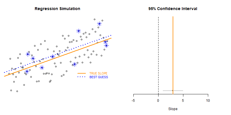
In this case we are taking repeated random draws of size N from a population, then calculating the slope and confidence interval of the slope. We want to note cases where b1 contains zero since these would represent NULL results in our study.
For a single sample we calculate the slope and confidence interval as follows:
# regression model: Y = b0 + b1(X)
d.sample <- dplyr::sample_n( d, size=N )
m <- lm( y ~ x, data=d.sample )
b1 <- (coef( m ))[2]
ci <- confint( m )
ci.b1.lower <- ci[2,1]
ci.b1.upper <- ci[2,2]
Then to examine lots of scenarios we can just repeat this code inside of a loop.
get_slope <- function( d, N=10 )
{
  d.sample <- dplyr::sample_n( d, size=N )
  m <- lm( y ~ x, data=d.sample )
  b1 <- (coef( m ))[2]
  ci <- confint( m )
  ci.b1.lower <- ci[2,1]
  ci.b1.upper <- ci[2,2]
  df <- data.frame( b1, ci.b1.lower, ci.b1.upper )
}

results <- NULL
for( i in 1:100 )
{
   one.model <- get_slope( d )
   results <- dplyr::bind_rows( results, one.model )
}
These types of bootstrapping simulations are very useful for generating robust versions of sampling statistics when the data is irregular or closed-form solutions do not exist.
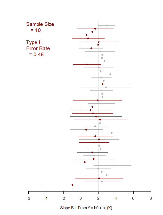
In this case were are interested in statistical power as a function of sample size. In studies like drug trials it might cost $10,000 for each study participant, so drug companies want to minimize the sample size needed to veryify the effectiveness of their drugs.
We can use previous research to ascertain a reasonable correlation between X and Y or anticipated effect size to simulate some population data.
Type II Errors represent cases that the regression fails to produce a slope that is differentiable from zero (the confidence interval of slope b1 contains zero).
We would start with a small sample size (n=10 in this example) then increase it until we have exceeded a target Type II Error rate.
Some helper functions were created to generate the proper statistics inside of the loops.
Pay attention to differences in the constructors.
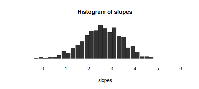
The first example collects only the slope from each simulation, so results are stored in a collector vector called slopes.
# BOOTSTRAPPING TYPE II ERRORS
# Examine Type II Errors
# as a function of sample size

# load data and helper functions
source( "https://raw.githubusercontent.com/DS4PS/cpp-527-fall-2020/master/lectures/loop-example.R" )
head( d )                       # data frame with X and Y
get_sample_slope( d, n=10 )     # returns a single value
test_for_null_slope( d, n=10 )  # returns a one-row data frame

## EXAMINE SLOPES
## sample size = 10


slopes <- NULL  # collector vector

for( i in 1:1000 )  # iterator i
{

  b1 <- get_sample_slope( d, n=10 )
  slopes[ i ] <- b1

}


# descriptives from 10,000 random draws, sample size 10

head( slopes )
[1] 2.246041 3.979462 1.714822 4.689032 1.763237 3.107451

summary( slopes )
#    Min. 1st Qu.  Median    Mean 3rd Qu.    Max.
#  -2.194   1.596   2.176   2.088   2.600   4.868

hist( slopes, breaks=25, col="gray20", border="white" )
The second example generates the slope, confidence interval (lower and upper bounds), and a null significance test from each new sample. The results are stored in a data frame called results.
## EXAMINE CONFIDENCE INTERVALS
## sample size = 10

# build the
# results data frame
# using row binding


results <- NULL

for( i in 1:50 )
{

  null.slope.test <- test_for_null_slope( d, n=10 )
  results <- rbind( results, null.slope.test )

}


head( results )

# confidence intervals from 50 draws, sample size 10

#            b1 ci.b1.lower ci.b1.upper null.slope
# x  -0.9783359  -4.5757086    2.619037       TRUE
# x1  2.3897431   0.4295063    4.349980      FALSE
# x2  2.0781628  -0.6677106    4.824036       TRUE
# x3  2.9178206   0.7080918    5.127549      FALSE
# x4  2.3702949   0.5238930    4.216697      FALSE
# x5  1.9701996   0.5513491    3.389050      FALSE

plot_ci( df=results )
## alternative constructor:
## the list version
## runs faster but it
## needs to be converted
## to a data frame afterwards

results <- list()

for( i in 1:50 )
{

  null.slope.test <- test_for_null_slope( d, n=10 )
  results[[ i ]] <- null.slope.test

}

## convert list to df
results <- dplyr::bind_rows( results )

head( results )
plot_ci( df=results )
Additional Reading
These readings are a slightly more advanced treatment of loops and control structures used in simulations. Dive in or bookmark them for later.