Week 02

Week 02

Q1 UNIT TESTING

We encountered a strange bug in the Monty Hall problem that arises from the behavior of the sample function in these scenarios:

# case a
sample( x=2, size=1, replace=FALSE )  # x turns into 1:2 or c(1,2)
# case b
sample( x=3, size=1, replace=FALSE )  # x turns into c(1,2,3)
# would not matter
sample( x=1, size=1, replace=FALSE )  # x is 1:1 so still just 1  

I have made the conjecture that this bug will result in the wrong door opened in 18% of games played.

In case A there is a 50% chance of returning the correct value from the sample function (random draw from [1,2] when the correct door is 2) and in Case B a 33% chance of returning the correct door (random draw from [1,2,3] when the correct door is 3).

We encounter each scenario 2 times out of 9: car in 1st position and we pick 3rd door, and vice-versa. Or car in second position and we pick 1st door, and vice-versa.

So we expect the error to occur in (2/9)(1/2) + (2/9)(1/3) = 0.185 proportion of games played.

Use the problematic open_goat_door() function below and write an automated unit test to measure the error rate at the stage of opening the goat door after the contestant makes the first selection (you don’t have to model the stay/switch step or final outcome step - you are only evaluating whether the correct door was opened here).

In your unit test visit each game scenario the same number of times (or approximately the same number).

# example scenarios - will be 9 total 
  
game <- c("goat","goat","car")
first.pick <- 1
correct.open.door <- 2

game <- c("goat","goat","car")
first.pick <- 2
correct.open.door <- 1

game <- c("goat","goat","car")
first.pick <- 3
correct.open.door <- c(1,2)

Play 10,000 games and compare the results of the open_goat_door() function to a set of correct outcomes (you will need to define these for each scenario).

Share your solution and report the average error rate of the function.

# PROBLEMATIC FUNCTION 
open_goat_door <- function( game, a.pick )
{
   doors <- c(1,2,3)
   available.doors <- doors[ game != "car" & doors != a.pick ] 
   opened.door <- sample( available.doors, size=1 )
   return( opened.door ) 
}

See the solutions from Lab 01 for some examples of writing unit tests.

Q2 - GAMBLING STREAKS AND DURATION MODELS

We covered a very basic animation in the lecture notes - a random walk.

Start game with $10 in cash. At each step you flip a coin and win a dollar, lose a dollar, or stay the same.

How long does it take for a player to lose all of their money?

While loops are useful when we repeat a process until a condition is met, the player being out of money in this case.

cash <- 10  
results <- NULL
count <- 1  
while( cash > 0 )
{
  cash <- cash +   
    sample( c(-1,0,1), size=1 )  
  results[count] <- cash  
  count <- count + 1  
}

Q2-A: Visualize the Game

Similar to the lecture notes, create a visualization of the cash that a player has at each round of the game until they go broke. Similar to this example but animated:

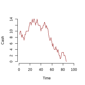
Q2-B: You’ve got to know when to fold them

Starting with $10 in the game, how long does it take the typical player to go bankrupt?

If you don’t want to do a complicated mathematical proof, create a simulation, play the game 10,000 times, then report the average duration of each game.

Would the mean or the median be a better measure of the average here?

I would suggest wrapping the code above into a play_game() function and calling that function repeatedly inside your loop.

Note: the interesting edge case in this simulation is a case where a person never goes broke so your program runs forever.

Is this a likely outcome when the players all start with $10?

How would you adapt your code to account for this scenario?

Q2-C: Finding Warren Buffet

If you run a simulation of 10,000 individuals playing the game, all starting with $10, how many individuals will never go broke?

Operationalize never in your code and explain your assumptions.

How many of these individuals did you find in your simulation?

Q3 - ANIMATIONS

A random walk is a one-dimensional outcome (cash in hand) tracked over time.

Physicists have used a similar model to examine particle movement with a Brownian Motion model.

It is similar to the betting model above except for each time period the particle moves in two dimensions.

x <- 0  
y <- 0 
for( i in 1:1000 )
{
  x[i+1] <- x[i] + rnorm(1)
  y[i+1] <- y[i] + rnorm(1)
}

Q3-A: Create the Brownian Motion animation above

Use the loop above to generate particle positions.

Create an animation to visualize the movement of the particle.

Discuss the package or app you used to generate the GIF.

Q3-B: Shadow of the past

If animations move too quickly it will look like popcorn and it can be hard to identify the meaningful patterns in the data.

You can enhance the information value of animations by visualizing change and in addition to the current model state include information on past stages.

How would you create the trailing tail in this animation?

Q4 CUSTOM ANIMATION

If you are not interested in Brownian Motion, share another animation you create using loops.

Do NOT simply find a package that has a pre-programmed animation.

Design your own animation using loops and explain your example.

You will, however, need a package (or external tool) to create a GIF from the animation.